Quickstart

Represent geometric path and trajectory

In TOPP-RA, both geometric paths \(\mathbf q(s)_{s \in [0, 1]}\) and parametrized trajectories \(\mathbf q(t)_{t \in [0, T]}\) are represented by classes that implement the abstract interface AbstractGeometricPath. The most important function is __call__() which can be used to evaluate the configuration, first-derivatives and second-derivatives respectively.

Spline Interpolator

In the examples, the child class toppra.SplineInterpolator is used extensively, due to the expressiveness and convenience offered by cubic spline. Note that this class is implemented as a thin wrapper over scipy’s CubicSpline. Therefore, it requires scipy to work properly. SplineInterpolator’s usage is simple.

>>> import toppra
>>> s_array = [0, 1, 2]
>>> wp_array = [(0, 0), (1, 2), (2, 0)]
>>> path = toppra.SplineInterpolator(s_array, wp_array)

That’s it. To verify that is works correctly, let’s try plotting.

>>> import numpy as np
>>> import matplotlib.pyplot as plt
>>> s_sampled = np.linspace(0, 2, 100)
>>> q_sampled = path(s_sampled)
>>> q_sampled[:2]
array([[0.        , 0.        ],
       [0.02020202, 0.07999184]])
>>> plt.plot(s_sampled, q_sampled); plt.show()  
[<matplotlib.lines.Line2D object at 0x...>, <matplotlib.lines.Line2D object at 0x...>]

You will see the following plot show up.

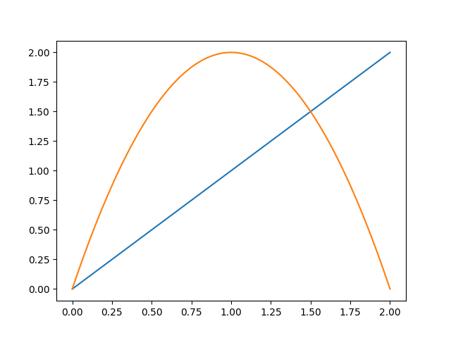
Geometric path plot.

The derivatives can be inspected by calling path(positions, order) using order=1 for the first derivative and order=2 for the second derivative respectively.

>>> q_dot = path(s_sampled, 1)
>>> q_ddot = path(s_sampled, 2)

Implement your own Interpolator

TOPP-RA can handle custom Interpolators easily, as long as it conforms to the abstract interface of toppra.interpolator.AbstractGeometricPath.

Retime geometric paths with parametrization

The parametrization step, given a fixed time-parametrization \(s(t)\) and a geometric path \(\mathbf{p}(s)\), is defined like so:

\[\begin{split}\mathbf q(t) &= \mathbf p(s(t)) \\ \dot{\mathbf p}(t) &= \mathbf p'(s) \dot s(t) \\ \ddot{\mathbf p}(t) &= \mathbf p'(s) \ddot s(t) + \mathbf p''(s) \dot s(t)^2\end{split}\]

toppra provides way to realize this step programmatically. Consider a simple geometric path

>>> import toppra
>>> path = toppra.SplineInterpolator([0, 1, 2], [(0, 0), (1, 2), (2, 0)])

Let’s consider a simple parametrization

>>> gridpoints = [0, 0.5, 1, 1.5, 2]
>>> velocities = [1, 2, 2, 1, 0]

We can quickly parametrize the geometric path with toppra:

>>> path_new = toppra.ParametrizeConstAccel(path, gridpoints, velocities)

Under the hood, ParametrizeConstAccel assumes that the path acceleration within each segment is constant. Combining with the function composition rule, the original is parametrized. ParametrizeConstAccel derives from AbstractGeometricPath and defines all specified methods such as computing the positions, derivatives and duration.

Any geometric path implementing the abstract geometric path interface can be used with ParametrizeConstAccel.

The parametrization can be inspected

>>> path_new.plot_parametrization(show=True)

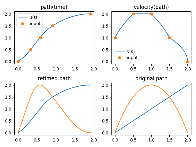
Parametrization.

>>> path_new(0)
array([0., 0.])
>>> path_new.path_interval
array([0.        , 1.91666667])

Trapezoidal Reparametrization

It’s common in automation and robotics to use trapezoidal velocity profile, or S-curve to make a movement more graceful. This can be easily implemented using the constant acceleration reparametrizer ParametrizeConstAccel.

See this code snippet below.

>>> path = toppra.SplineInterpolator([0, 2], [(0, 0), (1, 2)])
>>> gridpoints, velocities = (0, 0.25, 0.75, 1.0), (0, 1, 1, 0)
>>> path_new = toppra.ParametrizeConstAccel(path, gridpoints, velocities)
>>> path_new.plot_parametrization(show=True)

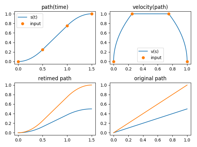
Parametrization.

TODO: It will be useful to have a collection of generators that generate these velocity profiles, based on the desired maximum velocity, duration, et cetera.

Time-optimal retime with kinematics constraints

The toppra algorithm returns the velocity profile, or the time-parametrization profile that is optimal. The resulting trajectory is also guaranteed to satisfy given constraints. Consider a simple path as below for a 2-dof robot.

>>> s_array = [0, 1, 2]
>>> wp_array = [(0, 0), (1, 2), (2, 0)]
>>> path = toppra.SplineInterpolator(s_array, wp_array)

Suppose the 2 dofs are constrained by velocity and acceleration limits.

>>> pc_vel = toppra.constraint.JointVelocityConstraint([[-1, 1], [-0.5, 0.5]])
>>> pc_acc = toppra.constraint.JointAccelerationConstraint([[-0.05, 0.2], [-0.1, 0.3]])

The time-optimal velocity profile can be found easily using TOPPRA

>>> instance = toppra.algorithm.TOPPRA([pc_vel, pc_acc], path)
>>> instance.compute_parameterization(0, 0)

Algorithm outputs are stored in the problem_data attribute:

>>> instance.problem_data.return_code
<ParameterizationReturnCode.Ok: 'Ok: Successful parametrization'>
>>> instance.problem_data.gridpoints  
array([0.      , 0.015625, 0.03125 , 0.046875, 0.0625  , 0.078125,...])
>>> instance.problem_data.sd_vec  
array([...])

>>> path_new = toppra.ParametrizeConstAccel(path, instance.problem_data.gridpoints, instance.problem_data.sd_vec)
>>> path_new.plot_parametrization(show=True)

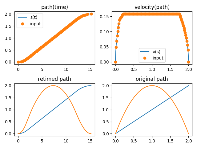
Parametrization.