Retime an one dimensional path

Import necessary libraries.

import toppra as ta
import toppra.constraint as constraint
import toppra.algorithm as algo
import numpy as np
import matplotlib.pyplot as plt

ta.setup_logging("INFO")

We now generate a simply path. When constructing a path, you must “align” the waypoint properly yourself. For instance, if the waypoints are [0, 1, 10] like in the above example, the path position should be aligned like [0, 0.1, 1.0]. If this is not done, the CubicSpline Interpolator might result undesirable oscillating paths!

waypts = [[0], [1], [10]]
path = ta.SplineInterpolator([0, 0.1, 1.0], waypts)

Setup the velocity and acceleration

vlim = np.array([[-3, 3]])
alim = np.array([[-4, 4]])
pc_vel = constraint.JointVelocityConstraint(vlim)
pc_acc = constraint.JointAccelerationConstraint(
    alim, discretization_scheme=constraint.DiscretizationType.Interpolation)

Setup the problem instance and solve it.

instance = algo.TOPPRA([pc_vel, pc_acc], path, solver_wrapper='seidel')
jnt_traj = instance.compute_trajectory(0, 0)

Out:

INFO [algorithm.py : 104] No gridpoint specified. Automatically choose a gridpoint with 129 points
INFO [algorithm.py : 191] Successfully parametrize path. Duration: 4.084, previously 1.000)
INFO [algorithm.py : 193] Finish parametrization in 0.006 secs

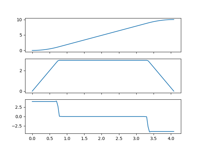
We can now visualize the result

duration = jnt_traj.duration
print("Found optimal trajectory with duration {:f} sec".format(duration))
ts = np.linspace(0, duration, 100)
fig, axs = plt.subplots(3, 1, sharex=True)
qs = jnt_traj.eval(ts)
qds = jnt_traj.evald(ts)
qdds = jnt_traj.evaldd(ts)
axs[0].plot(ts, qs)
axs[1].plot(ts, qds)
axs[2].plot(ts, qdds)
plt.show()

Out:

Found optimal trajectory with duration 4.083554 sec