Retime a path subject to kinematic constraints

In this example, we will see how can we retime a generic spline-based path subject to kinematic constraints. This is very simple to do with toppra, as we shall see below. First import the library.

import toppra as ta
import toppra.constraint as constraint
import toppra.algorithm as algo
import numpy as np
import matplotlib.pyplot as plt
import time

ta.setup_logging("INFO")

We generate a path with some random waypoints.

def generate_new_problem(seed=9):
    # Parameters
    N_samples = 5
    dof = 7
    np.random.seed(seed)
    way_pts = np.random.randn(N_samples, dof)
    return (
        np.linspace(0, 1, 5),
        way_pts,
        10 + np.random.rand(dof) * 20,
        10 + np.random.rand(dof) * 2,
    )
ss, way_pts, vlims, alims = generate_new_problem()

Define the geometric path and two constraints.

path = ta.SplineInterpolator(ss, way_pts)
pc_vel = constraint.JointVelocityConstraint(vlims)
pc_acc = constraint.JointAccelerationConstraint(alims)

We solve the parametrization problem using the ParametrizeConstAccel parametrizer. This parametrizer is the classical solution, guarantee constraint and boundary conditions satisfaction.

instance = algo.TOPPRA([pc_vel, pc_acc], path, parametrizer="ParametrizeConstAccel")
jnt_traj = instance.compute_trajectory()

Out:

INFO [algorithm.py : 104] No gridpoint specified. Automatically choose a gridpoint with 290 points
INFO [reachability_algorithm.py : 65] Solver wrapper not supplied. Choose solver wrapper automatically!
INFO [reachability_algorithm.py : 75] Select solver seidel
INFO [algorithm.py : 191] Successfully parametrize path. Duration: 3.525, previously 1.000)
INFO [algorithm.py : 193] Finish parametrization in 0.013 secs

The output trajectory is an instance of toppra.interpolator.AbstractGeometricPath.

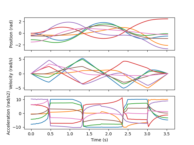
ts_sample = np.linspace(0, jnt_traj.duration, 100)
qs_sample = jnt_traj(ts_sample)
qds_sample = jnt_traj(ts_sample, 1)
qdds_sample = jnt_traj(ts_sample, 2)
fig, axs = plt.subplots(3, 1, sharex=True)
for i in range(path.dof):
    # plot the i-th joint trajectory
    axs[0].plot(ts_sample, qs_sample[:, i], c="C{:d}".format(i))
    axs[1].plot(ts_sample, qds_sample[:, i], c="C{:d}".format(i))
    axs[2].plot(ts_sample, qdds_sample[:, i], c="C{:d}".format(i))
axs[2].set_xlabel("Time (s)")
axs[0].set_ylabel("Position (rad)")
axs[1].set_ylabel("Velocity (rad/s)")
axs[2].set_ylabel("Acceleration (rad/s2)")
plt.show()

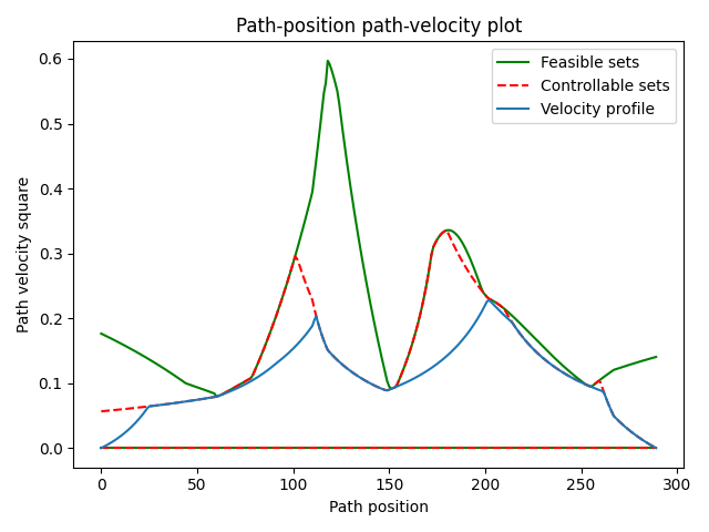
Optionally, we can inspect the output.

instance.compute_feasible_sets()
instance.inspect()